Understanding Macaulay Duration: A Practical Guide

When you hear investors talk about “duration,” they’re usually referring to the Macaulay duration—a cornerstone concept for anyone dealing with bonds. It condenses a bond’s cash‑flow schedule into a single number that reflects the weighted average time until you receive each payment. Grasping this idea helps you predict price changes, compare securities, and manage interest‑rate risk with far more confidence than a gut feeling ever could.

What Is Macaulay Duration and Why It Matters

At its core, Macaulay duration measures the time, in years, it takes for the present value of a bond’s cash flows to equal the bond’s price. Think of it as the “center of mass” of those cash flows. The longer the duration, the more sensitive the bond is to shifts in market interest rates. This makes the metric invaluable for portfolio managers who need to balance return expectations against potential volatility.

How to Calculate Macaulay Duration

The calculation involves three simple steps, but the arithmetic can feel a bit tedious without a spreadsheet.

• Identify each cash flow (coupon payments and principal) and the period in which it occurs.
• Discount each cash flow back to today using the bond’s yield to maturity (YTM). The formula is PV = CF ÷ (1 + YTM)^t, where t is the period number.
• Multiply each discounted cash flow by its time period, sum the results, and then divide by the bond’s current price.

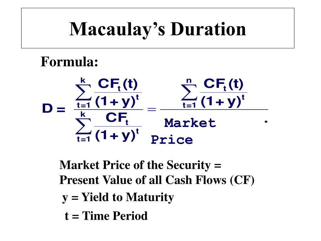
In formula form, Macaulay duration (D) looks like this:

D = ( Σ t × PV(CFₜ) ) ÷  Σ PV(CFₜ)

For example, imagine a 5‑year, 6 % annual coupon bond with a face value of $1,000, currently yielding 5 %. The cash flows are $60 each year and $1,060 at maturity. After discounting each payment, you’d weight them by the year they occur, add everything up, and finally divide by the bond’s price (about $1,045). The result is roughly 4.7 years—meaning the bond’s “average” cash‑flow timing sits just under five years.

Interpreting the Result: What Duration Tells You

A Macaulay duration of 4.7 years doesn’t mean the bond will be sold after that time; rather, it signals how the bond’s price will react to interest‑rate moves. A handy rule of thumb: for a small change in yield, the bond’s price will shift by approximately the duration multiplied by the change, expressed in percent.

Suppose yields climb by 0.25 %. A bond with a 4.7‑year duration would see its price drop by about 1.2 % (4.7 × 0.25 %). This linear approximation works best for modest rate shifts; larger moves require more sophisticated models.

Investors also compare Macaulay duration to modified duration, which adjusts for the bond’s yield compounding. Modified duration = Macaulay duration ÷ (1 + YTM/n), where n is the number of coupon periods per year. The modified version is the figure most traders actually use for price‑sensitivity calculations, but understanding the original Macaulay concept clarifies why the weighting by time matters in the first place.

Limitations and When Not to Rely Solely on Macaulay Duration

While Macaulay duration is elegant, it has blind spots. First, it assumes a flat yield curve—every cash flow is discounted at the same YTM. In reality, yields differ across maturities, so the measure can misstate risk for bonds with irregular cash‑flow patterns, such as mortgage‑backed securities.

Second, the metric treats all rate changes as parallel shifts. If the curve twists (short‑term rates rise while long‑term rates fall), the duration‑based estimate may be off. Third, for bonds with embedded options—callable or putable bonds—the cash‑flow schedule itself changes when rates move, rendering a static duration calculation less reliable.

Finally, duration captures only the first‑order effect of interest‑rate changes. For sizable moves, convexity becomes important; it measures the curvature of the price‑yield relationship and can either amplify or dampen the duration‑based prediction.

Practical Tips for Using Macaulay Duration in Portfolio Management

• Match Duration to Investment Horizon: Align the portfolio’s average duration with the time frame you expect to hold the assets. This reduces the risk of having to sell at an inopportune moment when rates have moved.
• Blend Bonds with Different Durations: Combining short‑ and long‑duration securities can smooth overall volatility while still achieving desired yield levels.
• Monitor Yield Curve Shifts: Keep an eye on whether changes are parallel or more complex. Adjust your holdings if you anticipate steepening or flattening trends.
• Use Duration as a Starting Point: Pair it with convexity, option‑adjusted spread (OAS), and scenario analysis for a fuller risk picture.

FAQ

What’s the difference between Macaulay and modified duration?

Macaulay duration expresses the weighted average time to receive cash flows, while modified duration adjusts that figure for the bond’s yield and directly estimates price sensitivity.

Can I use Macaulay duration for zero‑coupon bonds?

Yes. For a zero‑coupon bond, the Macaulay duration equals its maturity because there’s only one cash flow occurring at the end.

How does Macaulay duration handle semi‑annual coupons?

You treat each coupon period as a separate cash flow, discounting at the semi‑annual YTM (annual YTM divided by two) and counting periods in half‑years. The final duration will be expressed in years after dividing by the number of periods per year.

Is a higher duration always worse?

Higher duration means greater interest‑rate risk, but it also often accompanies higher yields. Whether it’s “worse” depends on your risk tolerance and market outlook.